In their famous article (see Learning Representations by Back-propagating Errors) Rumelhart, Hinton and Williams popularized the backpropagation mechanism in order to modify the weights of the links between neurons of different layers. They also added the momentum (parameter α alpha) to the classical learning rate (η eta) as a way to improve the Gradient Descent algorithm (learning mechanism). In this post, we will study the resulting learning curves of a MLP for the XOR function when modifying hyperparameters η(eta) and α(alpha).
Gradient Descent Algorithm
For an introduction to MLP, XOR and learning curve, see my previous post Capability of the MLP to learn XOR. For an overview of Deep Learning , see Deep Learning in Neural Networks: An Overview
For an introduction to Backpropagation and Gradient Descent or Stochastic Gradient Descent algorithm (SGD) see:
- Breaking down Neural Networks: An intuitive approach to Backpropagation
- Neural Networks: Feedforward and Backpropagation Explained & Optimization
- Wikipedia Backpropagation
- Intuitive Introduction to Gradient Descent
- Introduction to Stochastic Gradient Descent
- Wikipedia gradient descent
- Wikipedia Stochastic gradient descent
The MLP
For my tests, I chose to use a MLP with the tanh function as the activation function of the neurons. At the beginning of each training session, all the weights of each link from one neuron to the neurons of the next layer were set to a random value.
The cost function used is the mean squared error loss function (MSE).
Following Rumelhart, Hinton and Williams article, the weight of each link between neurons is updated using the following formula:
Δ Weight = η * ∇MSE + α * Preceding Δ Weight
New Weight = Old Weight + Δ Weight
I ran my tests using 2 topologies:
- 2 4 1 (2 neurons on the entry layer, 4 neurons on the hidden layer, 1 neuron on the output layer)
- 2 4 4 1 (2 hidden layers with 4 neurons on each layer)
Results of the tests
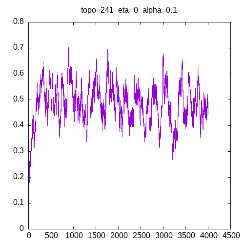
A picture being worth a 1000 words, let’s see the results for a 241 topology and η=0
As we can see, having a learning rate of 0 implies that the MLP seems unable to learn XOR function.
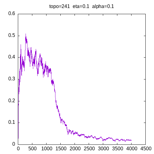
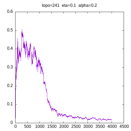
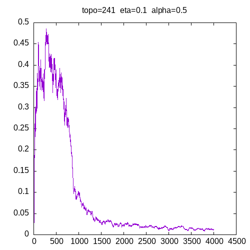
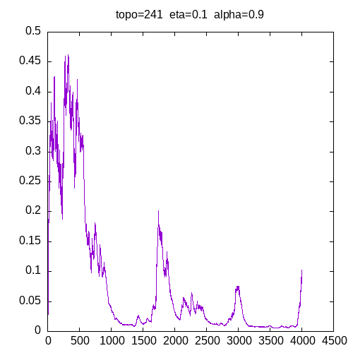
Let’s see now the learning curves for a 241 topology and η = 0.1
when α = 0.9, the learning curve starts to be irregular. when α = 1, the MLP seems unable to learn the XOR function.
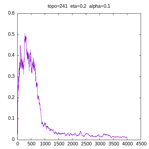
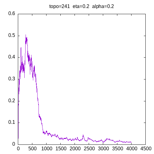
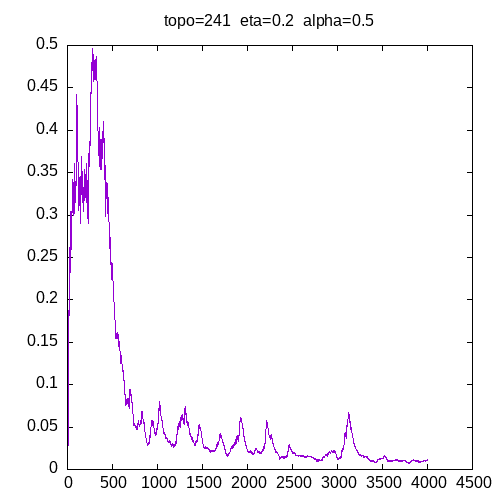
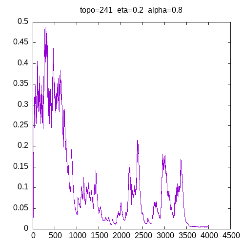
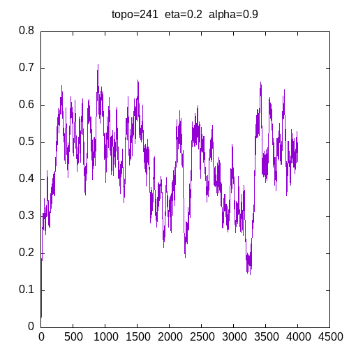
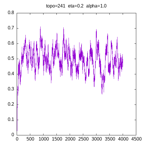
Let’s see the learning curves for a 241 topology and η=0.2
As we can see, for α > 0.9, the MLP seems unable to learn the XOR function. For α = 0.8 the learning curve is not smooth.
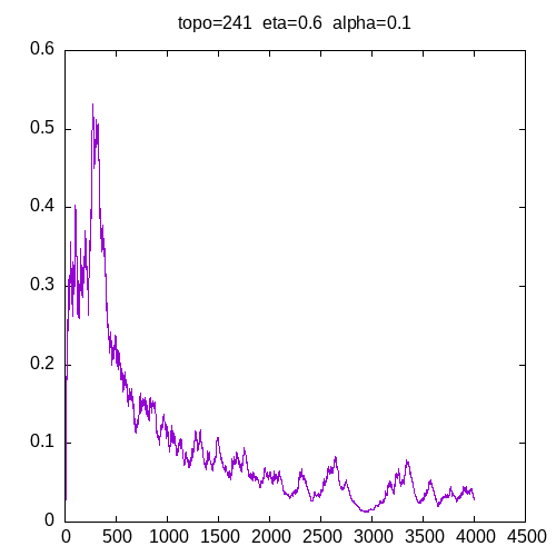
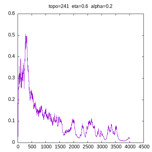
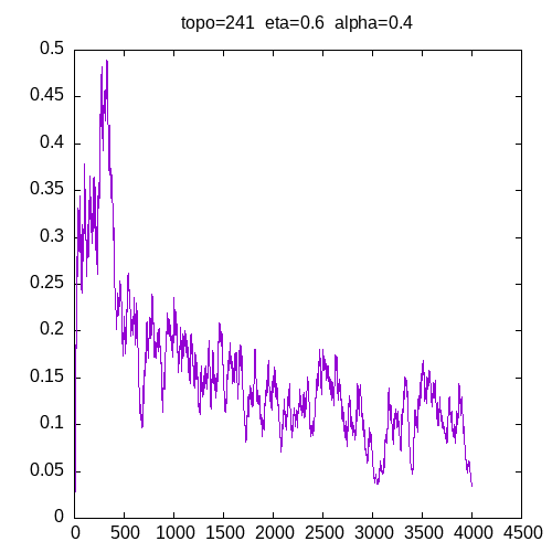
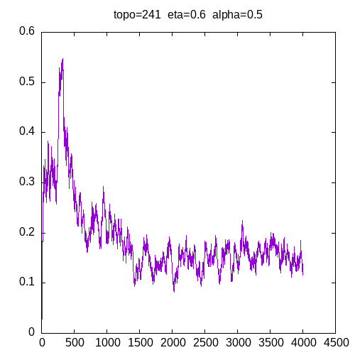
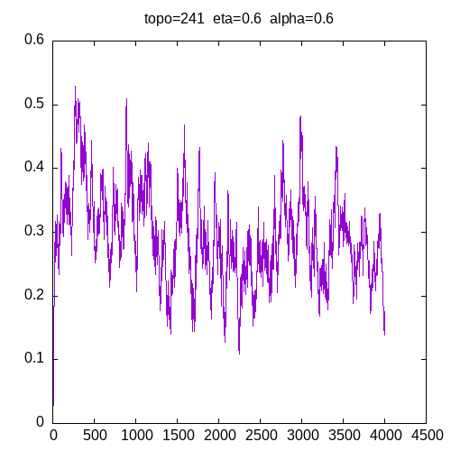
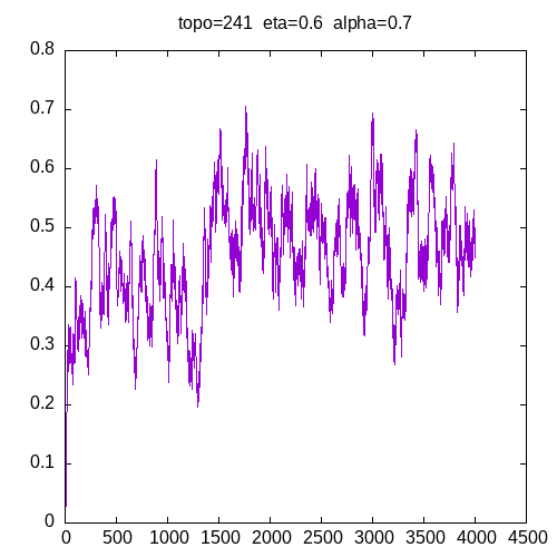
Let’s see the learning curves for a 241 topology and η=0.6
As we can see, for all alpha the learning curve is not smooth and for all α >= 0.6, the MLP seems unable to learn the XOR function.
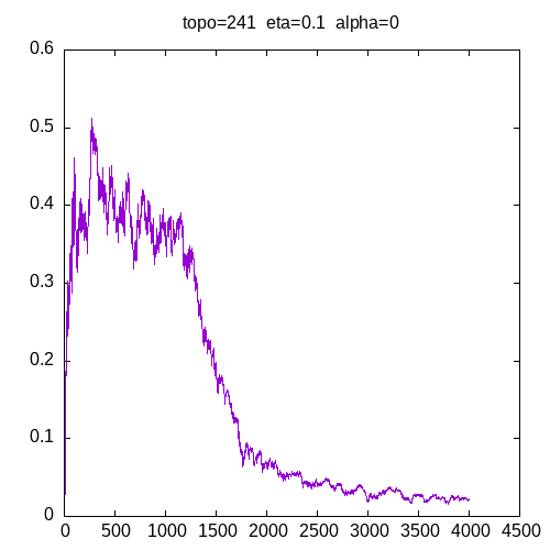
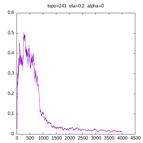
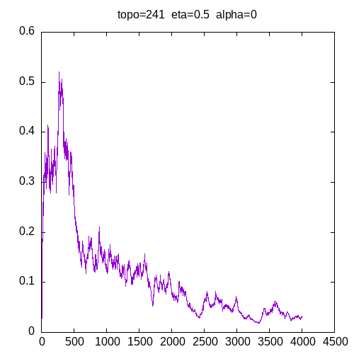
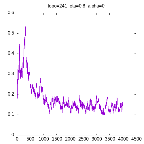
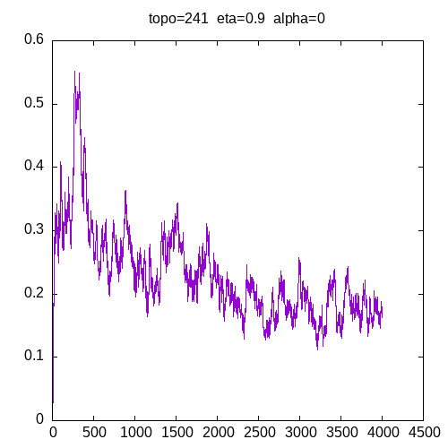
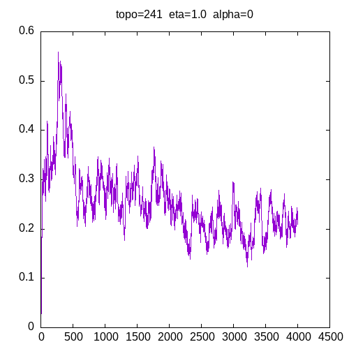
Let’s see the learning curves for a 241 topology and α=0
As we can see, the MLP is able to learn the XOR function but needs more entries in the training set as η increases. These graphs show that adding the α parameter improves the capability of the MLP to learn the XOR function.
In my next article, I will compare these results obtained for a 241 topology with the ones obtained for a 2441 topology.





1 thought on “Gradient Descent Algorithm: Impact of eta and alpha on the learning curve of MLP for XOR”